Simple active particle example
Here, we setup a simple 1D column example with the LOBSTER biogeochemical model and active particles modelling the growth of sugar kelp. This example demonstrates:
- How to setup OceanBioME's biogeochemical models
- How to add biologically active particles which interact with the biodeochemical model
- How to visualise results
This is forced by idealised mixing layer depth and surface photosynthetically available radiation (PAR) which are setup first.
Install dependencies
First we check we have the dependencies installed
using Pkg
pkg "add OceanBioME, Oceananigans, CairoMakie, JLD2"
Model setup
First load the required packages
using OceanBioME, Oceananigans, Printf
using Oceananigans.Fields: FunctionField, ConstantField
using Oceananigans.Units
using Oceananigans.Architectures: on_architecture

const year = years = 365days # just for these idealised cases
Surface PAR and turbulent vertical diffusivity based on idealised mixed layer depth
Setting up idealised functions for PAR and diffusivity (details here can be ignored but these are typical of the North Atlantic).
@inline PAR⁰(x, y, t) = 60 * (1 - cos((t + 15days) * 2π / year)) * (1 / (1 + 0.2 * exp(-((mod(t, year) - 200days) / 50days)^2))) + 2

@inline H(t, t₀, t₁) = ifelse(t₀ < t < t₁, 1.0, 0.0)

@inline fmld1(t) = H(t, 50days, year) * (1 / (1 + exp(-(t - 100days) / 5days))) * (1 / (1 + exp((t - 330days) / 25days)))

@inline MLD(t) = - (10 + 340 * (1 - fmld1(year - eps(year)) * exp(-mod(t, year) / 25days) - fmld1(mod(t, year))))

@inline κₜ(x, y, z, t) = 1e-2 * (1 + tanh((z - MLD(t))/10)) / 2 + 1e-4

@inline temp(x, y, z, t) = 2.4 * cos(t * 2π / year + 50day) + 10

architecture = CPU()Oceananigans.Architectures.CPU()Grid and PAR field
Define the grid and an extra Oceananigans' field that the PAR will be stored in
Lx, Ly = 20meters, 20meters
grid = RectilinearGrid(architecture, size=(1, 1, 50), extent=(Lx, Ly, 200))
1×1×50 RectilinearGrid{Float64, Periodic, Periodic, Bounded} on CPU with 1×1×3 halo
├── Periodic x ∈ [0.0, 20.0) regularly spaced with Δx=20.0
├── Periodic y ∈ [0.0, 20.0) regularly spaced with Δy=20.0
└── Bounded z ∈ [-200.0, 0.0] regularly spaced with Δz=4.0Specify the boundary conditions for DIC and O₂ based on the air-sea CO₂ and O₂ flux
CO₂_flux = CarbonDioxideGasExchangeBoundaryCondition()

clock = Clock(; time = 0.0)
T = FunctionField{Center, Center, Center}(temp, grid; clock)
S = ConstantField(35.0)ConstantField(35.0)Kelp Particle setup
@info "Setting up kelp particles"

n = 5 # number of kelp bundles
z₀ = [-21:5:-1;] * 1.0 # depth of kelp fronds

particles = SugarKelpParticles(n; grid,
                               advection = nothing, # we don't want them to move around
                               scalefactors = fill(2000, n)) # and we want them to look like there are 500 in each bundle

set!(particles, A = 10, N = 0.01, C = 0.1, z = z₀, x = Lx / 2, y = Ly / 2)
[ Info: Setting up kelp particles
Setup BGC model
biogeochemistry = LOBSTER(grid;
                          surface_PAR = PAR⁰,
                          inorganic_carbon = CarbonateSystem(),
                          detritus = CarbonNitrogenDissolvedParticulate(grid),
                          oxygen = Oxygen(),
                          scale_negatives = true,
                          particles)

model = NonhydrostaticModel(grid;
                            clock,
                            closure = ScalarDiffusivity(ν = κₜ, κ = κₜ),
                            boundary_conditions = (; DIC = FieldBoundaryConditions(top = CO₂_flux)),
                            biogeochemistry,
                            auxiliary_fields = (; T, S))

set!(model, P = 0.03, Z = 0.03, NO₃ = 4.0, NH₄ = 0.05, DIC = 2239.8, Alk = 2409.0)
Simulation
Next we setup the simulation along with some callbacks that:
- Show the progress of the simulation
- Store the model and particles output
- Prevent the tracers from going negative from numerical error (see discussion of this in the positivity preservation implementation page)
simulation = Simulation(model, Δt = 4minutes, stop_time = 150days)

progress_message(sim) = @printf("Iteration: %04d, time: %s, Δt: %s, wall time: %s\n",
                                iteration(sim),
                                prettytime(sim),
                                prettytime(sim.Δt),
                                prettytime(sim.run_wall_time))

simulation.callbacks[:progress] = Callback(progress_message, TimeInterval(10days))

filename = "kelp"
simulation.output_writers[:profiles] = JLD2Writer(model, model.tracers,
                                                  filename = "$filename.jld2",
                                                  schedule = TimeInterval(1day),
                                                  overwrite_existing = true)

simulation.output_writers[:particles] = JLD2Writer(model, (; particles),
                                                   filename = "$(filename)_particles.jld2",
                                                   schedule = TimeInterval(1day),
                                                   overwrite_existing = true)

qCO₂ = BoundaryConditionOperation(model.tracers.DIC, :top, model)

simulation.output_writers[:carbon_flux] = JLD2Writer(model, (; qCO₂),
                                                     indices = (:, :, grid.Nz),
                                                     filename = "$(filename)_carbon.jld2",
                                                     schedule = TimeInterval(1day),
                                                     overwrite_existing = true)
Run!
Finally we run the simulation
run!(simulation)[ Info: Initializing simulation...
Iteration: 0000, time: 0 seconds, Δt: 4 minutes, wall time: 0 seconds
┌ Warning: Attempting to store typeof(Main.var"##277".κₜ).
│ JLD2 only stores functions by name.
│ This may not be useful for anonymous functions.
└ @ JLD2 ~/.julia-oceananigans/packages/JLD2/qcxKY/src/data/writing_datatypes.jl:447
┌ Warning: Attempting to store typeof(Main.var"##277".κₜ).
│ JLD2 only stores functions by name.
│ This may not be useful for anonymous functions.
└ @ JLD2 ~/.julia-oceananigans/packages/JLD2/qcxKY/src/data/writing_datatypes.jl:447
┌ Warning: Attempting to store typeof(Main.var"##277".κₜ).
│ JLD2 only stores functions by name.
│ This may not be useful for anonymous functions.
└ @ JLD2 ~/.julia-oceananigans/packages/JLD2/qcxKY/src/data/writing_datatypes.jl:447
┌ Warning: Attempting to store typeof(Main.var"##277".κₜ).
│ JLD2 only stores functions by name.
│ This may not be useful for anonymous functions.
└ @ JLD2 ~/.julia-oceananigans/packages/JLD2/qcxKY/src/data/writing_datatypes.jl:447
┌ Warning: Attempting to store typeof(Main.var"##277".κₜ).
│ JLD2 only stores functions by name.
│ This may not be useful for anonymous functions.
└ @ JLD2 ~/.julia-oceananigans/packages/JLD2/qcxKY/src/data/writing_datatypes.jl:447
┌ Warning: Attempting to store typeof(Main.var"##277".κₜ).
│ JLD2 only stores functions by name.
│ This may not be useful for anonymous functions.
└ @ JLD2 ~/.julia-oceananigans/packages/JLD2/qcxKY/src/data/writing_datatypes.jl:447
┌ Warning: Attempting to store typeof(Main.var"##277".κₜ).
│ JLD2 only stores functions by name.
│ This may not be useful for anonymous functions.
└ @ JLD2 ~/.julia-oceananigans/packages/JLD2/qcxKY/src/data/writing_datatypes.jl:447
┌ Warning: Attempting to store typeof(Main.var"##277".κₜ).
│ JLD2 only stores functions by name.
│ This may not be useful for anonymous functions.
└ @ JLD2 ~/.julia-oceananigans/packages/JLD2/qcxKY/src/data/writing_datatypes.jl:447
┌ Warning: Attempting to store typeof(Main.var"##277".κₜ).
│ JLD2 only stores functions by name.
│ This may not be useful for anonymous functions.
└ @ JLD2 ~/.julia-oceananigans/packages/JLD2/qcxKY/src/data/writing_datatypes.jl:447
[ Info: ... simulation initialization complete (16.549 seconds)
[ Info: Executing initial time step...
[ Info: ... initial time step complete (3.578 seconds).
Iteration: 3600, time: 10 days, Δt: 4 minutes, wall time: 40.758 seconds
Iteration: 7200, time: 20 days, Δt: 4 minutes, wall time: 1.030 minutes
Iteration: 10800, time: 30 days, Δt: 4 minutes, wall time: 1.398 minutes
Iteration: 14400, time: 40 days, Δt: 4 minutes, wall time: 1.792 minutes
Iteration: 18000, time: 50 days, Δt: 4 minutes, wall time: 2.159 minutes
Iteration: 21600, time: 60 days, Δt: 4 minutes, wall time: 2.522 minutes
Iteration: 25200, time: 70 days, Δt: 4 minutes, wall time: 2.879 minutes
Iteration: 28800, time: 80 days, Δt: 4 minutes, wall time: 3.235 minutes
Iteration: 32400, time: 90 days, Δt: 4 minutes, wall time: 3.594 minutes
Iteration: 36000, time: 100 days, Δt: 4 minutes, wall time: 3.931 minutes
Iteration: 39600, time: 110 days, Δt: 4 minutes, wall time: 4.262 minutes
Iteration: 43200, time: 120 days, Δt: 4 minutes, wall time: 4.587 minutes
Iteration: 46800, time: 130 days, Δt: 4 minutes, wall time: 4.917 minutes
Iteration: 50400, time: 140 days, Δt: 4 minutes, wall time: 5.264 minutes
[ Info: Simulation is stopping after running for 5.622 minutes.
[ Info: Simulation time 150 days equals or exceeds stop time 150 days.
Iteration: 54000, time: 150 days, Δt: 4 minutes, wall time: 5.622 minutes
Now we can visualise the results with some post processing to diagnose the air-sea CO₂ flux - hopefully this looks different to the example without kelp!
tracers = FieldDataset("$filename.jld2")

air_sea_CO₂_flux = FieldTimeSeries(filename * "_carbon.jld2", "qCO₂")

x, y, z = nodes(tracers["P"])
times = tracers["P"].times
We compute the carbon export by computing how much carbon sinks below some arbirtrary depth; here we use depth that corresponds to k = grid.Nz - 20.
carbon_export = zeros(length(times))

using Oceananigans.Biogeochemistry: biogeochemical_drift_velocity

for (n, t) in enumerate(times)
    clock.time = t
    carbon_export[n] = tracers["sPOC"][n][1, 1, grid.Nz-20] * biogeochemical_drift_velocity(biogeochemistry, Val(:sPOC)).w[1, 1, grid.Nz-20] +
                       tracers["bPOC"][n][1, 1, grid.Nz-20] * biogeochemical_drift_velocity(biogeochemistry, Val(:bPOC)).w[1, 1, grid.Nz-20]
end
Both air_sea_CO₂_flux and carbon_export are in units mmol CO₂ / (m² s).
using CairoMakie

fig = Figure(size = (1000, 900), fontsize = 20)

axis_kwargs = (xlabel = "Time (days)", ylabel = "z (m)", limits = ((0, times[end] / days), (-85meters, 0)))

axP = Axis(fig[1, 1]; title = "Phytoplankton concentration (mmol N/m³)", axis_kwargs...)
hmP = heatmap!(times / days, z, interior(tracers["P"], 1, 1, :, :)', colormap = :batlow)
Colorbar(fig[1, 2], hmP)

axNO₃ = Axis(fig[2, 1]; title = "Nitrate concentration (mmol N/m³)", axis_kwargs...)
hmNO₃ = heatmap!(times / days, z, interior(tracers["NO₃"], 1, 1, :, :)', colormap = :batlow)
Colorbar(fig[2, 2], hmNO₃)

axD = Axis(fig[3, 1]; title = "Detritus concentration (mmol C/m³)", axis_kwargs...)
hmD = heatmap!(times / days, z, interior(tracers["sPOC"], 1, 1, :, :)' .+ interior(tracers["bPOC"], 1, 1, :, :)', colormap = :batlow)
Colorbar(fig[3, 2], hmD)

CO₂_molar_mass = (12 + 2 * 16) * 1e-3 # kg / mol

axfDIC = Axis(fig[4, 1], xlabel = "Time (days)", ylabel = "Flux (kgCO₂/m²/year)",
                         title = "Air-sea CO₂ flux and Sinking", limits = ((0, times[end] / days), nothing))
lines!(axfDIC, times / days, interior(air_sea_CO₂_flux, 1, 1, 1, :) ./ 1e3 * CO₂_molar_mass * year * 10, linewidth = 3, label = "Air-sea flux x10")
lines!(axfDIC, times / days, carbon_export / 1e3 * CO₂_molar_mass * year, linewidth = 3, label = "Sinking export")
Legend(fig[4, 2], axfDIC, framevisible = false)

save("kelp.png", fig)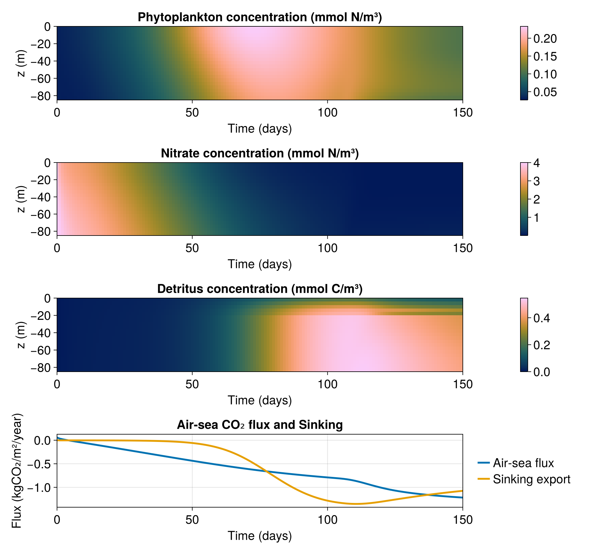
We can also have a look at how the kelp particles evolve
using JLD2

file = jldopen("$(filename)_particles.jld2")

iterations = keys(file["timeseries/t"])

A, N, C = ntuple(n -> zeros(5, length(iterations)), 3)

times = zeros(length(iterations))

for (i, iter) in enumerate(iterations)
    particles_values = file["timeseries/particles/$iter"]
    A[:, i] = particles_values.A
    N[:, i] = particles_values.N
    C[:, i] = particles_values.C

    times[i] = file["timeseries/t/$iter"]
end

Nₛ = particles.biogeochemistry.structural_nitrogen
Cₛ = particles.biogeochemistry.structural_carbon
kₐ = particles.biogeochemistry.structural_dry_weight_per_area
sf = particles.scalefactors[1]

fig = Figure(size = (1000, 800), fontsize = 20)

axis_kwargs = (xlabel = "Time (days)", limits = ((0, times[end] / days), nothing))

ax1 = Axis(fig[1, 1]; ylabel = "Frond area (dm²)", axis_kwargs...)
[lines!(ax1, times / day, A[n, :], linewidth = 3) for n in 1:5]

ax2 = Axis(fig[2, 1]; ylabel = "Total Nitrogen (gN)", axis_kwargs...)
[lines!(ax2, times / day, (@. A * (N + Nₛ) * kₐ * sf)[n, :], linewidth = 3) for n in 1:5]

ax3 = Axis(fig[3, 1]; ylabel = "Total Carbon (kgCO₂(eq))", axis_kwargs...)
[lines!(ax3, times / day, (@. A * (C + Cₛ) * kₐ * sf)[n, :] / 1000 * 44 / 12, linewidth = 3) for n in 1:5]

fig
This page was generated using Literate.jl.